dissmapr
A Novel Framework for Automated Compositional Dissimilarity and Biodiversity Turnover Analysis
1. Predict current Zeta Diversity (zeta2) using
predict_dissim()
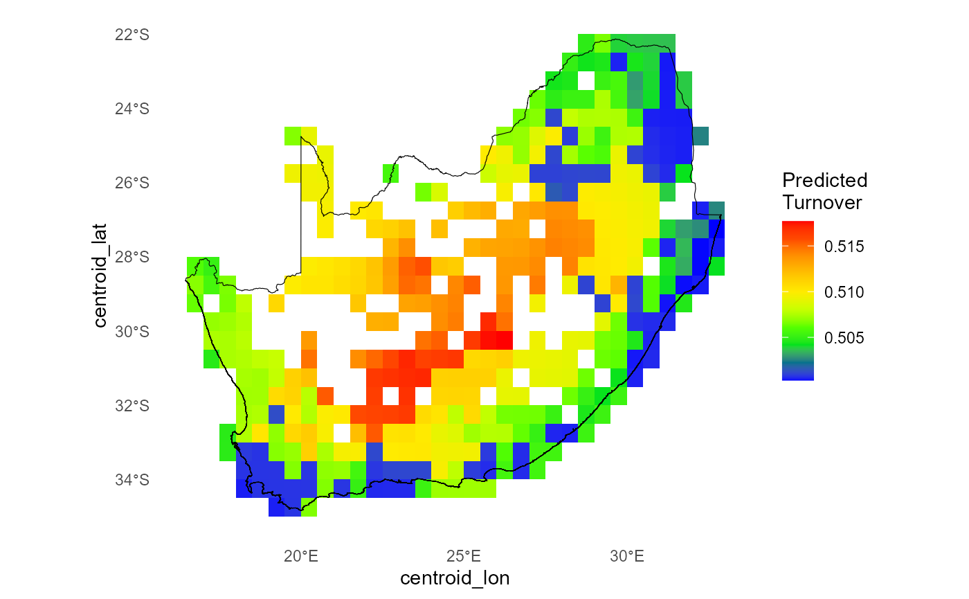
In this step we use our fitted order-2 GDM (zeta2) to
generate a spatial map of pairwise compositional turnover (ζ₂) under
current conditions. By calling predict_dissim() we
- compute each site’s sampling‐effort‐adjusted species richness and
mean distance to all other sites;
- apply the same environmental I-spline transformations used in the
model;
- predict the Jaccard-scaled turnover (ζ₂) on the 0–1 scale;
- optionally plot the resulting heatmap with your study boundary overlaid.
We set a random seed for reproducibility (so Monte Carlo sampling
inside predict_dissim() yields the same results each time),
pull out just the species columns once, then inspect the returned
predictors_df to confirm its dimensions, column names, and
a quick peek at the key model outputs.
# Predict current zeta diversity using `predict_dissim` with sampling effort, geographic distance and environmental variables
# Only non-colinear environmental variables used in `zeta2` model
set.seed(123) # set.seed to generate exactly the same random results i.e. sam=100
spp_cols = names(grid_spp_pa[,-(1:7)])
predictors_df   = predict_dissim(
  grid_spp      = grid_spp_pa,
  species_cols  = spp_cols,
  env_vars      = env_vars_reduced,# env_vars_reduced[,-8]
  zeta_model    = zeta2, # From simple order 2 run above
  # zeta_model = ispline_gdm_tab$zeta_gdm_list[[1]], # From list of Zeta.msgdm models
  grid_xy       = grid_env,
  x_col         = "centroid_lon",
  y_col         = "centroid_lat",
  bndy_fc       = rsa, # Optional feature collection to plot as boundary
  show_plot     = TRUE
)
# Check results
dim(predictors_df)
#> [1] 415  14
names(predictors_df)
#>  [1] "temp_mean"        "iso"              "temp_wetQ"        "temp_dryQ"
#>  [5] "rain_dry"         "rain_warmQ"       "obs_sum"          "distance"
#>  [9] "richness"         "pred_zeta"        "pred_zetaExp"     "log_pred_zetaExp"
#> [13] "centroid_lon"     "centroid_lat"
head(predictors_df[,5:11])
#>    rain_dry  rain_warmQ    obs_sum distance richness  pred_zeta pred_zetaExp
#> 1 -1.227648 -0.17604221 -0.2926985 903.0437        2 0.01930100    0.5048251
#> 2 -1.223151 -0.11642238 -0.2340532 915.4655       31 0.02632131    0.5065799
#> 3 -1.154108  0.06618959 -0.2818954 931.1100       10 0.01570100    0.5039252
#> 4 -1.149209  0.38933728 -0.2865253 949.9390        7 0.01506016    0.5037650
#> 5 -1.080356  0.62285852 -0.2880686 971.8672        6 0.01472191    0.5036804
#> 6 -1.048567  0.57126837 -0.1321955 996.7561       76 0.01438702    0.5035967
2. Predict future Zeta Diversity using
predict_dissim()
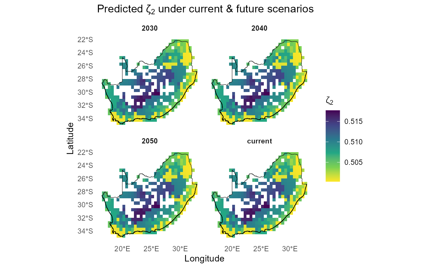
Below we expand our workflow to forecast how ζ₂ respond to three extreme climate futures (2030, 2040, 2050) alongside the current scenario.
First, we define and center-scale each future by adding large temperature increments and rainfall multipliers, then bundle them into a named list of four environmental data frames:
# 1. Identify species & env columns
# spp_cols  = names(grid_spp_pa)[-(1:7)]
all_vars  = names(env_vars_reduced)
temp_vars = grep("^temp", all_vars, value = TRUE)
rain_vars = grep("^rain", all_vars, value = TRUE)
iso_vars = grep("^iso", all_vars, value = TRUE)
obs_var = "obs_sum"

# 2. Extreme future shifts
horizons     = c("2030","2040","2050")
mean_delta   = list(
  temp  = c("2030"= +2,  "2040"= +4,  "2050"= +6),
  iso   = c("2030"= +0.5,"2040"= +1.0,"2050"= +1.5),
  rain  = c("2030"= 0.9, "2040"= 0.8, "2050"= 0.7),
  effort= c("2030"= 1.3, "2040"= 1.6, "2050"= 2.0)
)
exagg_factor = c("2030"=1.5, "2040"=2.0, "2050"=2.5)

# 3) helper to amplify deviation from the mean
amplify = function(x, factor) {
  m = mean(x, na.rm=TRUE)
  m + (x - m) * factor
}

# # 4. Save original scaling parameters
# sc_params = scale(env_vars_reduced)
# mu    = attr(sc_params, "scaled:center")
# sigma = attr(sc_params, "scaled:scale")

# 4. Build list of future env tibbles
env_scenarios = c(
  list(current = env_vars_reduced),
  map(horizons, function(yr) {
    df = env_vars_reduced
    # mean shifts
    df[temp_vars] = df[temp_vars] + mean_delta$temp[yr]
    df[iso_vars]  = df[iso_vars]  + mean_delta$iso[yr]
    df[rain_vars] = df[rain_vars] * mean_delta$rain[yr]
    df[[obs_var]] = df[[obs_var]] * mean_delta$effort[yr]
    # amplify spatial variation
    df[temp_vars] = map_dfc(df[temp_vars], amplify, factor = exagg_factor[yr])
    df[iso_vars]  = map_dfc(df[iso_vars],  amplify, factor = exagg_factor[yr])
    # clamp obs_sum
    df[[obs_var]] = pmin(pmax(df[[obs_var]], 50), 8000)
    df
  }) |> set_names(horizons)
)
# names(env_scenarios) = names(horizons)

# 5. Prepend current conditions
# env_scenarios = c(list(current = env_vars_reduced), env_futures)
str(env_scenarios, max.level = 1)
#> List of 4
#>  $ current: tibble [415 × 7] (S3: tbl_df/tbl/data.frame)
#>  $ 2030   : tibble [415 × 7] (S3: tbl_df/tbl/data.frame)
#>  $ 2040   : tibble [415 × 7] (S3: tbl_df/tbl/data.frame)
#>  $ 2050   : tibble [415 × 7] (S3: tbl_df/tbl/data.frame)
Next, we loop through each scenario, re-apply the original centering
and scaling, and call our predict_dissim() helper to
compute ζ₂. We tag each result with its scenario name and combine them
into one tidy data frame:
set.seed(123)

scenario_dfs = purrr::imap(env_scenarios, ~ {
  df = predict_dissim(
    grid_spp     = grid_spp,
    species_cols = spp_cols,
    env_vars     = .x,
    zeta_model   = zeta2,
    grid_xy      = grid_env,
    x_col        = "centroid_lon",
    y_col        = "centroid_lat",
    skip_scale   = FALSE,
    show_plot    = FALSE
  )
  df$scenario = .y
  df
})
str(scenario_dfs, max.level=1)
#> List of 4
#>  $ current:'data.frame': 415 obs. of  15 variables:
#>  $ 2030   :'data.frame': 415 obs. of  15 variables:
#>  $ 2040   :'data.frame': 415 obs. of  15 variables:
#>  $ 2050   :'data.frame': 415 obs. of  15 variables:

# all_preds = bind_rows(scenario_dfs) %>%
#   mutate(scenario = factor(scenario, levels = c("current", names(temp_shifts))))
all_preds = bind_rows(scenario_dfs)
head(all_preds)
#>   temp_mean         iso temp_wetQ temp_dryQ  rain_dry  rain_warmQ    obs_sum
#> 1  1.841044  0.05124962  1.426512 0.5759178 -1.227648 -0.17604221 -0.2926985
#> 2  1.770287 -0.16040417  1.434249 0.5279913 -1.223151 -0.11642238 -0.2340532
#> 3  1.888447  0.23118933  1.406438 0.6828768 -1.154108  0.06618959 -0.2818954
#> 4  2.222843  0.75512585  1.510132 0.9797353 -1.149209  0.38933728 -0.2865253
#> 5  2.424011  1.38701985  1.551582 1.1832058 -1.080356  0.62285852 -0.2880686
#> 6  2.809129  1.80976342  1.766238 1.4127484 -1.048567  0.57126837 -0.1321955
#>   distance richness  pred_zeta pred_zetaExp log_pred_zetaExp centroid_lon
#> 1 903.0437        3 0.01930100    0.5048251       -0.6835432        28.75
#> 2 915.4655       41 0.02632131    0.5065799       -0.6800731        29.25
#> 3 931.1100       10 0.01570100    0.5039252       -0.6853275        29.75
#> 4 949.9390        7 0.01506016    0.5037650       -0.6856454        30.25
#> 5 971.8672        6 0.01472191    0.5036804       -0.6858133        30.75
#> 6 996.7561      107 0.01438702    0.5035967       -0.6859795        31.25
#>   centroid_lat scenario
#> 1    -22.25004  current
#> 2    -22.25004  current
#> 3    -22.25004  current
#> 4    -22.25004  current
#> 5    -22.25004  current
#> 6    -22.25004  current
We can then quickly compare the spatial ζ₂ surfaces under each future:
ggplot(all_preds,
       aes(centroid_lon, centroid_lat, fill = pred_zetaExp)) +
  geom_tile() +
  facet_wrap(~ scenario, ncol = 2) +
  scale_fill_viridis_c(direction = -1, name = expression(zeta[2])) +
  geom_sf(data = rsa, fill = NA, color = "black", inherit.aes = FALSE) +
  coord_sf() +
  labs(x = "Longitude", y = "Latitude",
       title = expression("Predicted ζ"[2] * " under current & future scenarios")) +
  theme_minimal() +
  theme(strip.text = element_text(face = "bold"),
        panel.grid = element_blank())